Unlocking EV Power Consumption Secrets: The LeoINAGPS System
Measuring electric vehicle (EV) power consumption is crucial, but what if you could also track it in relation to the route, gradients, and altitudes? This innovative project makes it possible to detect basic electrical parameters of the traction motor and correlate them with the route, using a GPS receiver and Google Maps.
The Inspiration Behind the Project
A friend of mine, who uses an electric scooter for mobility, inspired this project. Living in a mountainous region with frequent steep climbs and descents, his scooter’s lead-acid batteries need to be replaced often. I wondered how much the scooter consumed in various conditions, considering an upgrade to high-performance lithium-ion batteries. The scooter features a heavy DC permanent-magnet motor and lead-acid batteries, unlike modern ebikes and scooters with compact, lightweight brushless motors and lithium batteries.
The LeoINAGPS System
I modified an existing system for measuring direct current (DC) load consumption to include a GPS receiver, allowing me to save the vehicle’s position and speed on a microSD card. This system can be applied to all electric vehicles, with adjustments to the shunt and voltage adapter. By tracking power consumption in relation to the route, we can gain valuable insights into EV performance and optimize battery life.
For the GPS, I used my own functions to read speed, position, and UTC time. I discarded the GPS altitude reading, which has insufficient accuracy to derive the slope of the climbs. During the first compilations of the new program, I realized that the RAM (2 kB) of the Arduino Nano ATMega328 MCU was insufficient for stable operation. I thought, therefore, to replace it with an ATmega32U4 MCU like the one used on Arduino Leonardo. It has 2.5 kB of RAM and a free UART.
The name of this project comes partly from Leonardo (the board is Arduino Leonardo-compatible), from the INA226 name of the module which measures the current and voltage on the load, and from the GPS receiver that completes the system.
From these tests, I derived the power consumption of the scooter, driven by my friend, in the various conditions of the route easily identifiable from the Google map. Unfortunately, the slope was not calculated from the GPS vertical coordinate because it has insufficient accuracy and resolution. There are pressure sensors that can provide the altitude with a resolution of a few tens of centimeters, but these were not used in the tests.
System Description
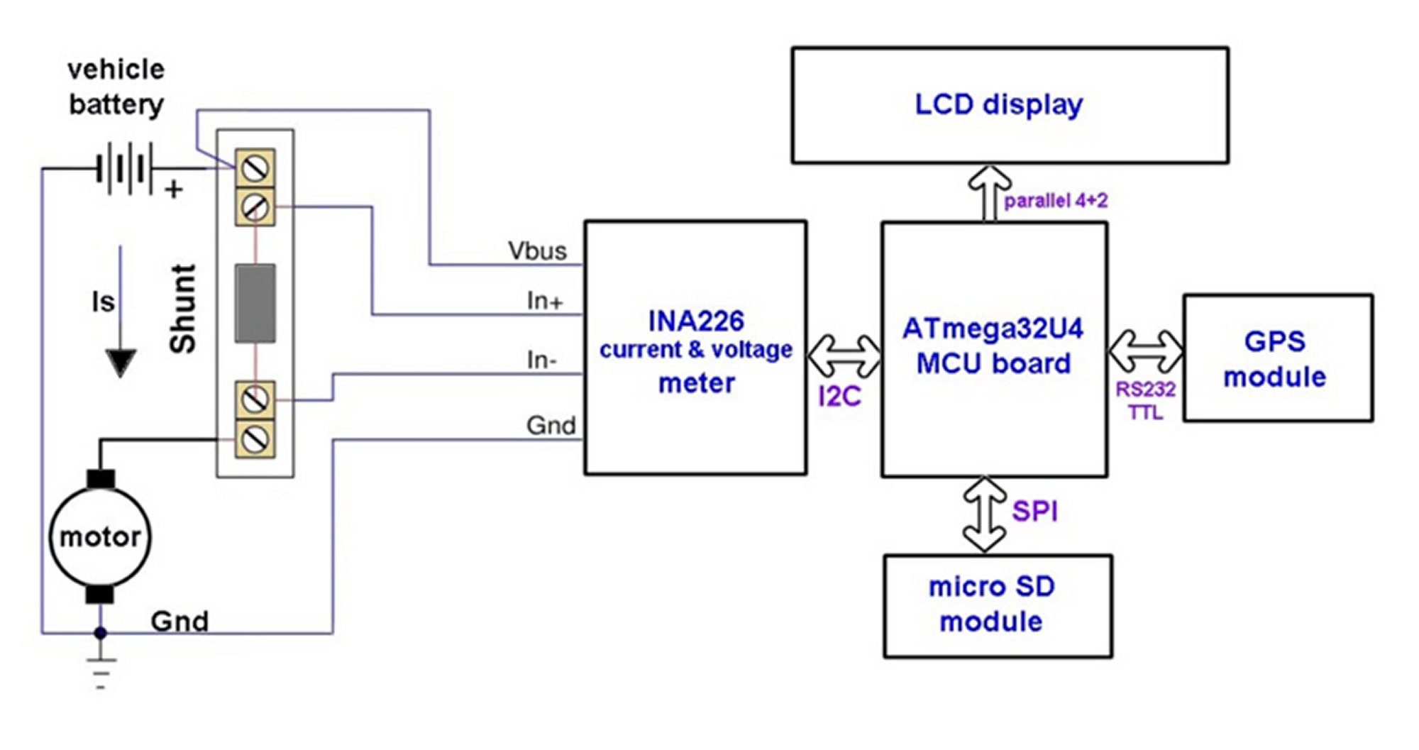
The functional diagram of the various components that compose the system is shown in Figure 1.
The INA226 Module
In current measurements with the shunt, there are two ways to insert it:
- Toward ground (low-side): The shunt is connected between the load and the ground.
- Toward source (high-side): The shunt is connected between the power supply source and the load.
The INA226 integrated circuit, by Texas Instruments, is a digital device that measures the current with a high-side or low-side shunt and also measures the voltage, calculates the power and provides a multifunctional alarm span>. The INA226 functional scheme is visible in Figure 2.
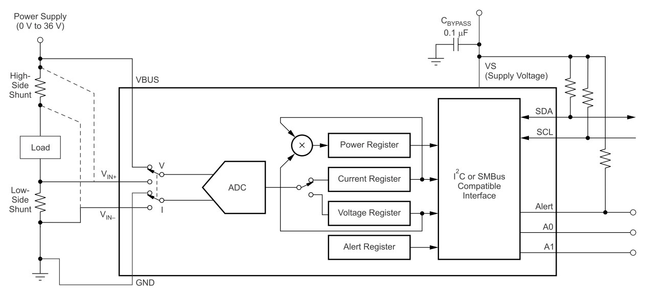
The internal ADC is based on a 16-bit delta-sigma converter (ΔΣ) with a typical conversion time of a few milliseconds, so it is also suitable for currents that change rapidly over time. It can also measure negative currents — negative numbers are represented in two’s complement format.
The resolution of the shunt voltage is 2.5 µV with a full scale of 32,768 × 2.5 µV = 81.92 mV. For the VBUS voltage, the resolution is 1.25 mV with a theoretical full-scale of 40.96 V, even if the 36 V must not be exceeded. The resolution of the power is 25 times that of the current, with the full scale depending on the shunt used. So, the system has a remarkable measurement accuracy.
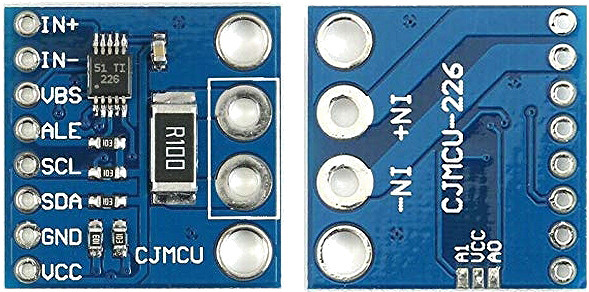
The chip is interfaced with the MCU via I2C bus. Small modules (breakout boards) like the one I used, visible in Figure 3, can be found on the market. The device has two address pins, A0 and A1, connecting them to VCC, GND, SDA, or SCL determines the I2C address of the INA226. The module I used mounts two pull-down resistors, so the address is 0x40. There are pads on the back to change it: By connecting them to VCC or SDA or SCL you can get up to 16 different addresses, which is very useful for monitoring a battery with many cells.
This module mounts a 0.1 Ω shunt (R100) that allows the measurement of a maximum current of 0.8192 A. But I preferred to remove it, soldering a 1 µF capacitor in its place as a noise filter, and to use my own shunt (more on this below).
The ATmega32U4 Pro Micro Module
The Pro Micro module used has an MCU type ATmega32U4 and is Arduino Leonardo-compatible. It can be programmed with the Arduino IDE by setting the Leonardo board. The whole thing is tiny: about 33 × 18 mm, even smaller than the Arduino Nano, which is similar to that of an old 24 pin DIL EPROM. If you don’t have space problems, an Arduino Leonardo board can be used instead.
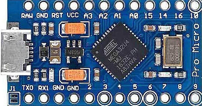
Figure 4 shows the board used for the project. The board I used has a 5 V regulator and can be powered via USB or from the RAW input (6…12 V). If we feed from the RAW pin with a minimum voltage of 6 V, the VCC is +5 V, produced by the regulator. If we feed from the USB, +4.8 V is available on RAW, a decreased value due to the dropping of a Schottky diode, which has a protection function, together with a fuse. If one wanted to use the internal regulator, which has no heat sink, I recommend using low voltages of 6…7.2 V and avoiding connecting loads above 100…150 mA. If an external regulator is available, as in our case, the board can also be powered with +5 V at the VCC pin by excluding the internal regulator.
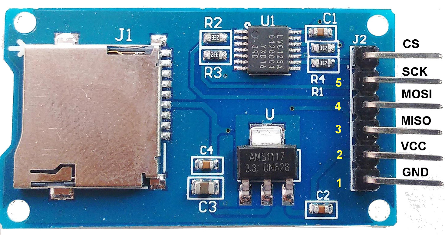
The MicroSD Module
I chose an SD module suitable for Arduino, i.e., with 5 V logic levels and a 5 V power supply; its appearance can be seen in Figure 5. It mounts a 3.3 V regulator and a level adapter. Modules without level adapters and the 3.3 V regulator should not be used for this project. To manage the SD, I used Arduino’s SD library.
The LCD
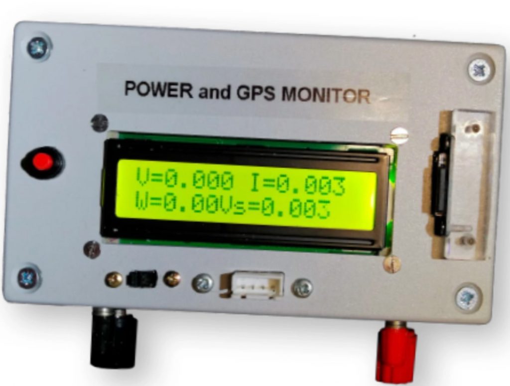
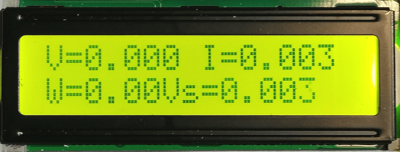
I used a common two-line 16-character LCD with a Hitachi HD44780-compatible controller and a backlit equipped with high-efficiency LED diodes that consumed about 20 mA, which I reduced to 10 mA by inserting an external resistor in series with the internal one. In Figure 6, we see the appearance of the display which is connected to the MCU with a parallel interface with 4 data and 2 control bits.
The GPS Module
There are numerous GPS/GNSS satellite receivers on the market, even at low cost. The important thing is that it can be powered at 5 V and you also need to know the baud rate of the serial port, which is normally 4,800 or 9,600 bit/s. Some modules have a built-in antenna, others have a discrete one. I used an old 4,800 baud receiver, with built-in antenna and magnetic base, and a 4-pin JST connector to wire it to the system.
Circuit Diagram
Figure 7 (see next page) shows the schematic of the system. In addition to the connector for the serial interface, I also mounted a switch to select power measurements, with or without GPS. The SS button is used to start or stop the acquisition on microSD. The LM7805 regulator could also be eliminated if we use the one on the board, but the external one is definitely more reliable, which in this case requires a minimum voltage of 7 V and — if equipped with a heatsink — can work up to 24 V. The current draw of the instrument (with backlighting) is about 47…50 mA.
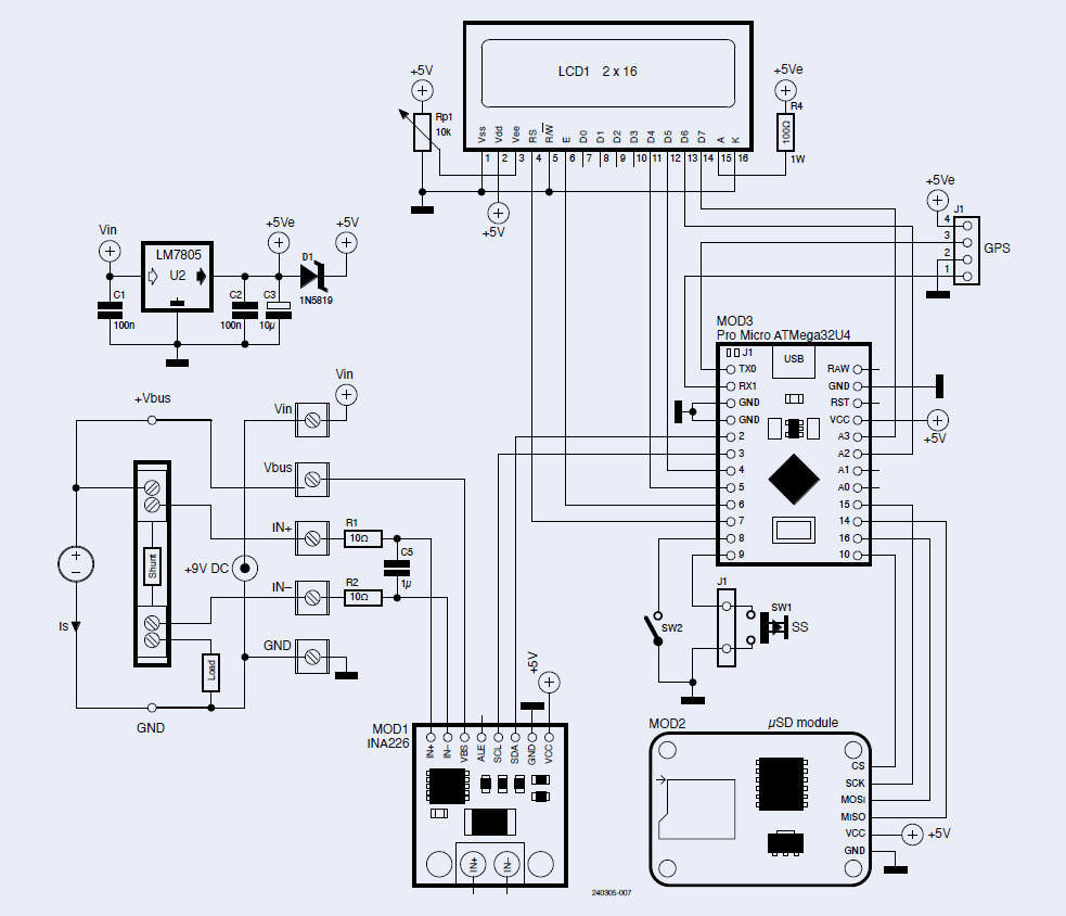
Schottky diode D1 avoids the conflict that would occur in the case in which the external power supply (5Ve) and USB power are both present. Resistors R1 and R2, together with capacitor C5, form a first-order low-pass filter to reduce noise.
Shunt Calculation
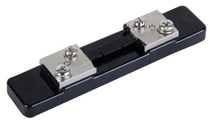
For high currents, it is best not to resort to self-building the shunt: 10, 20, 50, and 100 A ranges or more are easily found on the market. They are also very accurate, typically ranking in the 0.5% class and look similar to Figure 8. A fairly common voltage value at the shunt output terminals is 75 mV, for all full-scale currents.
This full-scale voltage is very close to that one of the INA226, which is 81.92 mV. In my case, I wanted to measure currents up to 50 A and with the 75 mV shunt; therefore, its resistance is:
Rse = 75 mV / 50 A = 1.5 mΩ
The full-scale current now becomes:
Ifs = 81,92 mV / Rse = 54.613 A
The resolution of the current will be:
54.613 / 32768 = 1.666 mA
The maximum power, dissipated by the shunt, will be:
P = V * I = V2 / R = 4.474 W
GPS Data
For the interpretation of the NMEA messages, transmitted by the GPS receiver, I used functions written by me. The program reads the NMEA RMC (Recommended Minimum Specific Data) sentences as, in addition to the position coordinates, it also contains the speed, expressed in knots, and date and time. For example:
$GPRMC,141507.870,A,4429.2796,N,00907.4338,E,0.00,,180522,,*1B
That means UTC time: 14:15:07.870, valid data, latitude 44°29.2796’ N, longitude 9°07.4338’ E, speed 0 knots, no course, date 18/05/2022, no mode indicator. The parameters are shown in Table 1.
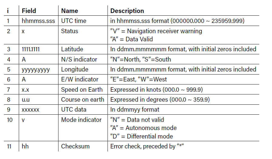
Coordinates are converted from degrees and minutes to decimal degrees, and the string outdata, saved to microSD, is organized as follows:
,time,latitude,longitude,speed
And, in the case of the previous example:
,141507,4429.2796,00907.4338,0.00
INA226 Management Software
I used a modified version of Korneliusz Jarzebski’s INA226.h library, as there were some errors in the original. I modified the functions calibrate(float rShunt, float iMaxExpected) and setShuntVoltageLimit(float voltage).
Perhaps it has now been modified by the author, but I recommend using the version available for download at the Elektor Labs webpage for this article, since it has been tested with this system.
The calibrate() function has as input parameters the shunt resistance and the maximum current, in our case:
rShunt = 0.0015 Ω and iMaxExpected = 54.613 A
It calculates several variables:
- currentLSB = iMaxExpected / 32768 = 54.613 / 32,768 = 1.666 [mA]
- calibrationValue = 0.00512 / currentLSB / rShunt = 0.00512 / 0.00166 / 0.0015 = 2,048
- powerLSB = currentLSB * 25 = 0.000625 * 25 = 15.625 [mW]
The Display and microSD Data Formats
Considering the resolution of the variables to be printed on the display, these are their formats:
- Bus voltage: V=xx.xx (7 characters)
- Shunt current: I=xx.xxx (8 characters)
- Bus power: W=xxx.xx (8 characters printed)
So, on the first line, I enter the voltage and current, separated by a space, and on the second line I enter the power, like this:
V=xx.xx I=xxx.xxx
W=xx.xx
In case GPS is used, the speed in km/h and UTC time are shown on the second line.Power Consumption Measurements
The string dataString, which will be saved to SD, is organized as follows:
Vbus,Ishu,power,Vshu
Where Vbus is the battery voltage, Ishu is the current flowing through the shunt, power is their product and Vshu is the voltage at the ends of the shunt. If GPS is not on board, these are the only measurements for each sampling; if GPS is present, time, position and speed data will also be added.
LeoINAGPS System Tests
For these tests, I used the 50 A shunt described above, which is 0.5% class. These tests were carried out in a small village in the Ligurian Apennines, and the instrumentation was mounted on an electric mobility scooter, visible in Figure 9, driven by its owner, my friend Roberto. To make room for the instrumentation, the casing under the driver’s seat was removed.
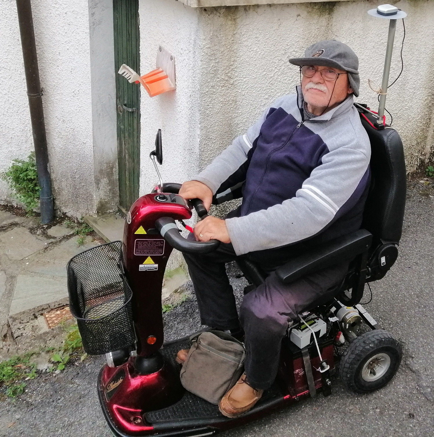
Roberto visibly concerned about the modifications made to his vehicle!
The route started from the garden of my friend’s house, the first part being characterized by several descents, more or less steep, while the return was done on another road with fairly steep climbs. There were, however, several sections walked in both directions. The route was relatively short but with rather steep inclines that put a strain on the engine of these scooters, which are mostly Chinese-built.
They are equipped with a conventional DC motor of about 1,000 W, powered by two 12 V lead-acid batteries suitable for electric traction, connected in series. Protection consists of a 40 A fuse and a 30 A thermal switch. The onboard MOSFET-based electronic controller drives the motor in PWM mode. The original batteries had a capacity of 35 Ah, but were replaced with 45 Ah ones to increase the range on non-flat terrain such as the test area. Batteries, on such a mountainous terrain, have a relatively short life and need to be replaced almost every year. Actually, the indicated capacity of 45 Ah is calculated on a 20-hour discharge (I = 2.25 A), and for a 5-hour discharge, a condition closer to the real one, it is reduced to 35 Ah (I = 7 A).
Except for the GPS, the instrumentation was mounted under the seat of the scooter and on top of the batteries, as seen in Figure 8 and Figure 10. The LeoINAGPS system was powered by two lithium batteries in series (7.2 V).
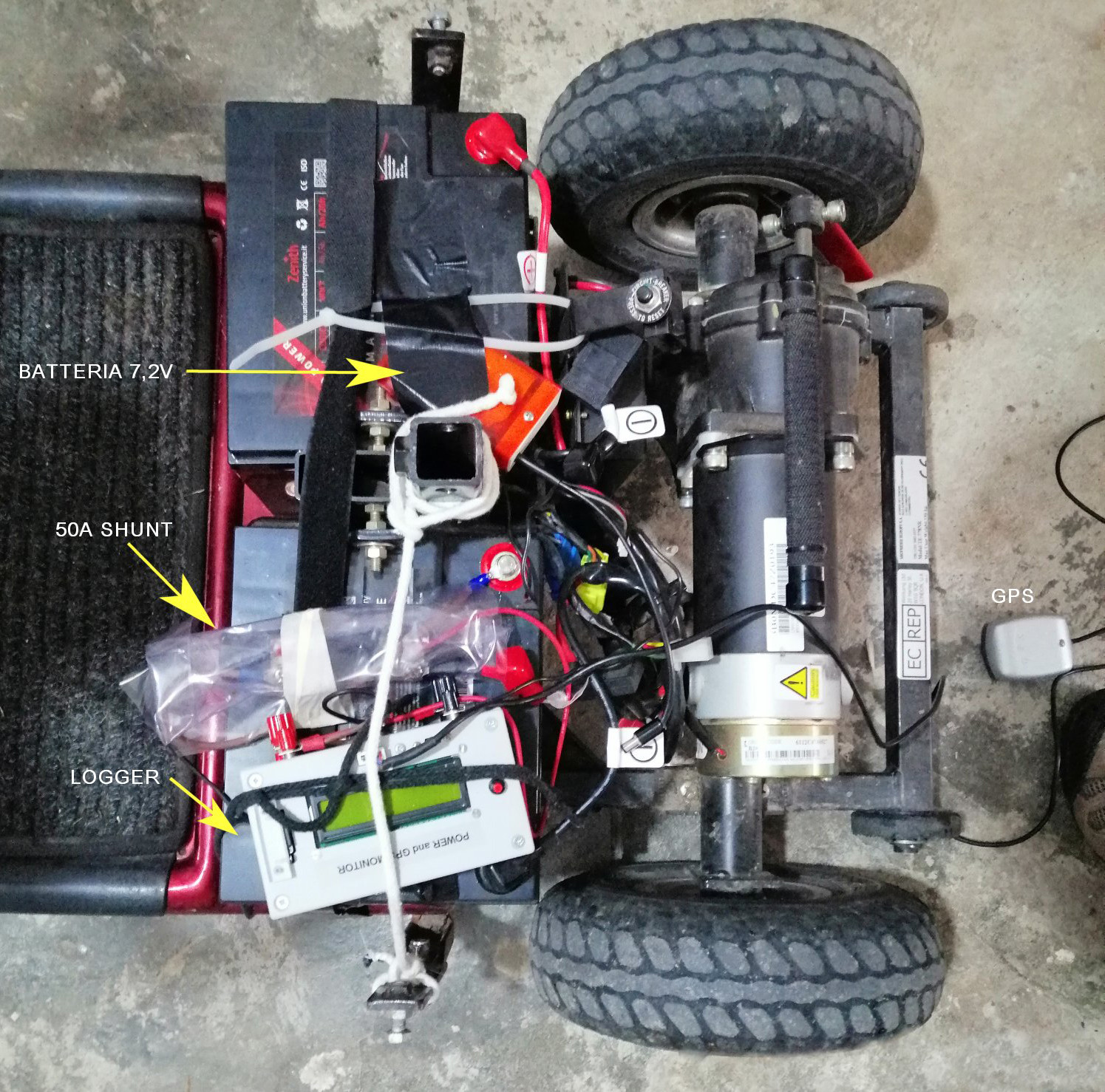
The GPS receiver was mounted on a special stand so as not to be obstructed by the driver, as seen in Figure 9, it incorporates antenna and receiver. GPS receivers usually provide a position measurement every second, so the system must be synchronized with the reception of NMEA messages. Each measurement, saved on the microSD card, consists of eight pieces of data: battery voltage [V], current delivered [A], power [W], shunt voltage [V], UTC time, latitude, longitude, and speed [km/h]. Coordinates are expressed in degrees and tenths of a degree.
Before starting acquisition by pressing the button on the front of the logger, one must wait for the GPS to receive and process the signal coming from at least three satellites, which takes a few minutes. When the GPS is up and running, the LED starts flashing, and the UTC time also appears on the display.
Italian local time is one hour ahead of UTC during daylight savings / summer time (CEST) or two hours head during standard time (CET). When the tests are finished, the button must be pressed again to end the acquisition. The test went very well and lasted 963 s, about 16 minutes.
Measurements: Power Consumption and More
Figure 11 shows time-history plots of battery voltage, current delivered, power and speed of the vehicle as a function of time, expressed in seconds. The section where the speed is null is because the vehicle stopped to take the picture shown in Figure 9. On descents, the brush motor acts as a dynamo and, in these sections, the current reversed and the voltage exceeded 32 V a few times, which is not ideal for the batteries.
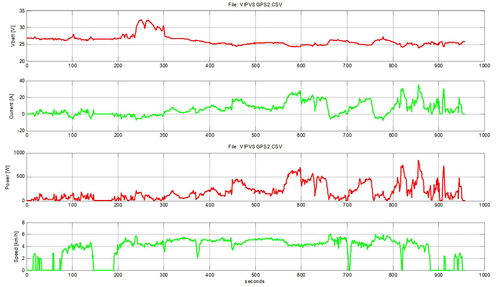
Important information is obtained from the time-history current graph, from which one can easily recognize the various descents, identified by the negative current values: the first descent (instants 89…112) then a small bump and the beginning of the second descent (instant 136) followed by the stop (instants 148…186) and the continuation with various downhill slopes (instants 189…300), the longest, the third (660…683) and the fourth (759…786), the most intense.
As was to be expected, the highest consumption occurred at the climbs, with peaks of more than 800 W. You can see the current peaks when starting the engine or stopping the scooter (brakes).
The typical speed during the test was about 4 to 5 km/h with some peaks of 6 km/h, practically similar to walking pace. This is because there were no long flat stretches. The outward run ended at instant 372; the return run was done on a largely different route and was also longer. The moment of reversal can be seen in the speed diagram as a spike from 5.2 down to 2 km/h. This maneuver can be seen even better from the longitude plot, shown in Figure 12.
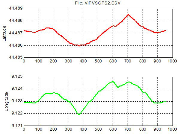
The scooter, after a fairly steep climb, took a small road that it traveled for a hundred meters and then returned. This reversal, which occurred at instant 704, can be seen in the latitude plot. From these curves, we can see that the coordinates of the end point are similar to the starting point.
Importing the Route Into My Maps
To see the route superimposed on the satellite photos, one can use My Maps and Google Maps, which are available online and completely free. You need to have a Google account and follow these simple steps:
- On your computer, log in to My Maps.
- Click on +CREATE A NEW MAP.
- In the map legend, click on Add layer.
- Give the new layer a name if you like.
- In the new layer, click Import.
- Choose or upload the VIPVSGPS.csv file and click Select.
- Select the columns containing latitudes (the first), longitudes (the second), and labels for each point (e.g., power).
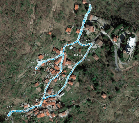
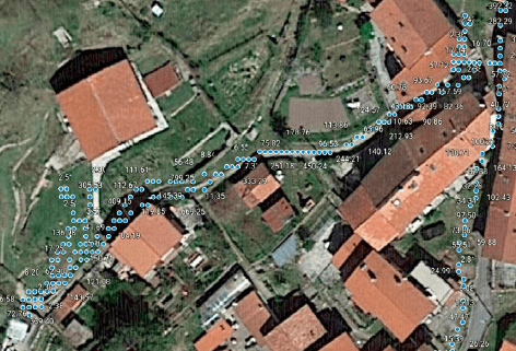
If you want to see the route with Google Maps and overlay the satellite photo, just import the layer with simple operations. The result is shown in Figure 13, and Figure 14 shows only the detail where the route began and ended. These programs allow you to place a certain value next to each point, in this case I preferred to indicate the power measured on the engine at that instant.
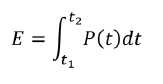
Energy Calculation
One important thing to get an idea of the range is to know how much energy has been drawn from the batteries. The amount of electrical energy ∆E supplied by the batteries to the motor depends on the power developed and the time ∆t = t2 – t1; if the power P were constant over time, the energy would be easily calculated:
∆E = P•∆t [J] (1)
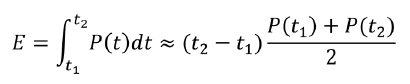
Energy in the international system is expressed in joules (1 J = 1 W/s); for electrical systems we prefer to use Watt-hours (Wh), obtained by dividing by 3,600. In our case, the power is not constant at all but varies over time, so we have to go from discrete to continuous and formula (1) becomes:
A basic numerical method of performing an integration is that of trapezoids:
This system is quite approximate. To make the definite integral of a function — that is, the area subtended — one replaces P(t) with many trapezoids, the area of which is easy to calculate, as shown in Figure 15.
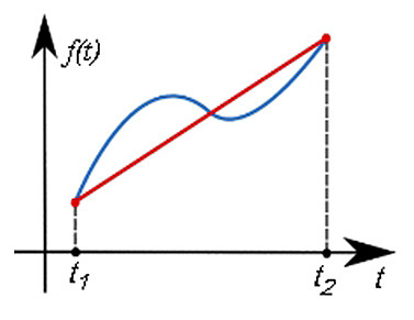
This method is more accurate as the ∆t decreases. In our case, the sampling period, ∆t, is one second, so:
E2 = (P1 + P2) ∙ 1s / 2 + E1 [J]
With a spreadsheet, it is easy to calculate the energy in J and, dividing by 3,600, in Wh. To estimate the approximate range of the scooter, we need to calculate the charge C lost by the accumulators, expressed in Ah, we need to integrate the current, similarly to what we saw for energy, so:
C2 = (I1 + I2) ∙ 1s / 2 + C1 [Ah]
The charge is related to the energy by the voltage; in fact, the energy in [Wh] is obtained by multiplying the charge with the average voltage. The results of the test data, processed in Matlab, are the following:
- LeoINAGPS system measurement processing.
- Processed file name = VIPVSGPS2.CSV
- Number of samples acquired = 963
- Sampling period = 1.000 [s]
- Energy supplied to the motor = 48.943 [Wh]
- Lost capacity (P&N) = 1.650 [Ah]
- Lost capacity (P) = 1.793 [Ah]
- Average battery voltage = 26.103 [V]
- Average discharge current = 6.206 [A]
- Capacity (E/V Average) = 1.875 [Ah]
In this case, the lost capacity (positive & negative) is underestimated, partly because of the too high ∆t and partly because of the stretches where the current is negative (slopes), which do not effectively contribute to the battery charging. In fact, in the end they are more harmful, than useful. Capacity calculated only on positive current (P), average battery voltage, and average current were also calculated.
The Program
At startup, the program initializes the I/O, LCD display, INA226, checks if the microSD card is present, and reads the position of the GPS switch. In setup(), the serial port is initialized with a baud rate of 4,800:
Serial1.begin(4800); // initialize UART with GPS baud rate
If your module is more modern, it is likely to have a baud rate of 9,600, in which case you need to change that function parameter.
When you set the switch to GPS, the program sends ”Wait for GPS ..” to the display and waits for a valid signal coming from the GPS. The GetData() function is the one that extracts the time, position, and speed from the NMEA RMC sentences.
When the data are valid (Status = “A”) the speed and time (hhmmss) appear on the second line of the display. This function also converts the coordinates, originally expressed in degrees and minutes, to the notation in decimal degrees.